Iannix + Csound: A Parametric Music System
Project Overview
This project explores the integration of IanniX’s visual graphing capabilities with Csound’s synthesis engine. The final result is a parametric music system which utilizes the contour lines of a 3D shape, programmed within the IanniX system, to inform oscillator parameters within a constrained musical system in Csound. The control capabilities within IanniX allow for the resulting composition to not only be a static, generative piece, but also an interactive system that encourages the user to distort the original parameters to explore the sonic relationships defined within the space.
When both systems are running, IanniX serves as an interactive visualization for the musical environment within Csound. As the piece develops, the user will see individual cursors moving along the contour lines defined in IanniX which each have mapped the x, y, and z parameters to distinct variables within the audio synthesis process.
Graphing in Iannix
IanniX scores generate data by making use of three primary graphing tools: lines, cursors, and events. The lines are simply lines defined somewhere in the 3D space and control where the cursors move along. The cursors represent the elements of the score that change continuously throughout time, and can be placed along lines to move across throughout the composition. The events can also be placed anywhere in 3D space, and are used to send binary trigger data, being triggered by cursors colliding with their definable boundary.
Generating a Möbius Strip
For this project, the goal was to model an interesting shape that would both look interesting, and yield interesting data output for audio. I decided on a Möbius strip, which is notable for being a one-sided 3D object. Since a Möbius Strip exists as a 2D plane within 3D space, modeling it in IanniX isn’t completely straightforward since IanniX is really only built for 1-dimensional lines/curves. My solution was to generate contour lines that would resemble a Möbius Strip when placed contiguously. This was a straightforward task since IanniX easily allows curves to be defined via parametric equations, and since a Möbius Strip is most aptly defined via parametric equations, this suited my situation perfectly.
Parametric Equations in IanniX
The term Parametric can seem kind of daunting to an uninitiated listener; however, in the context of this program it becomes pretty straightforward. A parametric equation is one whose spatial coordinates (x, y, and z in our case) are defined by an outside variable instead of the explitict $y = x$ relationship. In IanniX, we are granted the ability to define curves parametrically, allowing us to write independant equations for each dimension. We can use this to come up with interesting shapes by simply combining simple or complex equations for each coordinate. Furthermore, these equations can be written with params, which automatically create variable sliders which can be used to transform the resulting shape through the variable’s defined influence on the function throughout the performance.
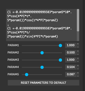
If you are interested in trying this out for yourself, I’d recommend adding a math curve within the default curves in IanniX; this creates a sine wave shape across the x and y-axis. By selecting the curve and going to the info → 3D Space tab, you can see the equation that defines the curve in an editable box, along with params which are written into the equation. By playing around with this and editing it with some different equations, you can get a solid grasp of what parametric equations are, and how to utilize them within IanniX.
Mobius Strip Equation
In order to implement curves for the Möbius strip, we will need to know the parametric equations that define it. These are listed below.
\[\begin{aligned} x(u,v) = (R + v\cos\frac{u}{2})\cos{u} \\ y(u,v)= (R + v\cos\frac{u}{2})\sin{u} \\ z(u,v)= v\sin\frac{u}{2} \\ \end{aligned}\]Each equation defines one of the dimensional coordinates for the Möbius strip, $x, y, z$. Since this is parametric, this is ideal for IanniX which expects a parametric equation. However, in order to draw this in IanniX, we need to breakdown this equation a bit further so we can isolate which variables we will need to parameterize in the equations.
Writing a Curve Function
We can try loading this equation straight into a curve within IanniX if we replace each variable $R, u, v$ with IanniX’s slider parameter keyword param. Here, param1 will become the variable $R$, param2 becomes $v$, and param3 becomes $u$. Each variable has been scaled by $4\pi$ to create a complete effect.
( param1 * 3.14 * 4 + param2 * 3.14 * 4 * cos(param3 * 3.14 * 4 * t / 2) ) * cos(param3 * 3.14 * 4 * t),
( param1 * 3.14 * 4 + param2 * 3.14 * 4 * cos(param3 * 3.14 * 4 * t / 2) ) * sin(param3 * 3.14 * 4 * t),
( param3 * 3.14 * 4 * sin(param1 * 3.14 * 4 * t / 2)
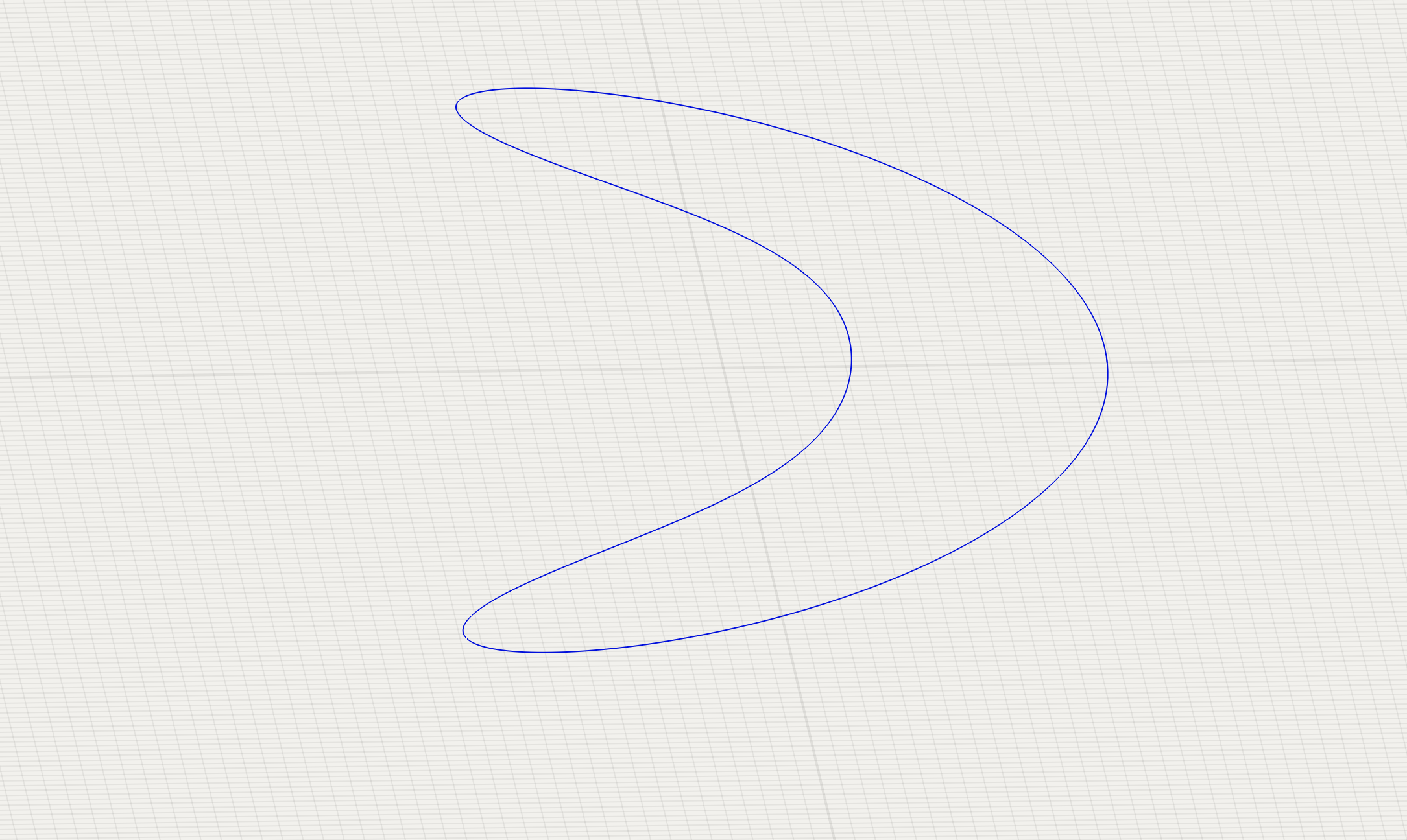
By adjusting the parameter values, we can generate a curve like the one shown below. Param1 controls the radius of the Möbius strip, while param2 and param3 represent the parametric variables that evolve over time to define its shape. Sliding these parameters reveals how the Möbius strip-like form emerges from the curve boundaries. This insight provides our approach: by generating multiple curves with the same parametric equations but incrementally varied parameter values, we can create a series of contour lines that collectively outline a Möbius strip in 3 dimensions. However, manually creating and adjusting at least 20 individual curves would be tedious. Fortunately, IanniX’s script editor offers an efficient solution.
Scripting in Iannix
Iannix provides a scripting editor in a javascript like languages with a series a built in commands to control Iannix parameters. These commands include generating curves, lines, triggers, and cursors; modifying their functions; and performing other more general operations. For this overview, I’ll avoid going into too much detail about the general scripting language and instead focus on what I did to generate the Mobius strip. More information on the scirpting commands can be found within the Iannix Software Documentation.
mobius() Function
Below shows a general function I came up with for creating the mobius strip. This can be run simply by placing within in the provided default function, makeWithScript(). There is some additional functionality included in this example, but most of those are self-explanatory, and are merely for aesthetics.
Most of the generation for the Möbius strip is happening within the for loop. To start, we need to know how many curves we are going to generate, and across what boundaries we want our strip to be defined. This is done with the Num_Curves variable. Here, Num_Curves is hard-coded into the script; however, it can optionally and usefully be loaded as a chosen variable by the user by adding it in the default askUserForParameter() function.
The v variable
The variable we are going to iterate across to produce our strips is v. This is the same as the $v$ variable in the original Möbius equation, and will represent the width of the Möbius strip. Since this can also be a useful variable, it has been defined above with the other user variables, and added into the equation as parameter 5. We use this width variable to obtain the increment value for v by dividing the width by Num_Curves.
Within the for loop, we begin executing many of the run("...") commands that actually perform tasks within the IanniX program. First, a curve is created, along with an ID we increment thoughout the loop. The curve is then added to the ‘mobius’ group, and its position and size (which more closely corresponds to thickness for curve lines) are set.
IDs and Groups
There are a few useful considerations to note when generating many functions like this. IanniX gives curves an ID number to help identify specific curves, added when generated. As well as this, objects can be added into groups that allow you to perform common operations on all group members at once. This is extremely useful for these cases where we are using 20+ curves for one specific function. Adding a curve to a group within the scripting is simple too; in this case, it is done with a single command: run("setgroup current mobius");, where mobius corresponds to a variable group name.
setEquation()
Finally we get to the setEquation() function, where the bulk of the interesting things are happening. The format for the setEquation command is
setEquation current polar_flag x_equaiton, y_equation, z_equation
Since we have to set 3 complex equations within one line, we end up with the unwieldly looking command below…
setEquation current 0 (1 +" + v + "*param5*10*.5*cos(4*PI*t*2 * param1))*cos(t*4*PI*param2),(1 +" + v + "*param5*10*.5*cos(4*PI*t/2*param3))*sin(4*PI*t*param4)," + v +"*param5*10* 0.5 * sin(4*PI*t/2)
If we breakdown one of the equation commands, we can see how easily it maps onto the original mobius equation. The parametric equation for the x-dimension is as follows…
\[x(u,v) = (R + v\cos\frac{u}{2})\cos{u} \\\]This becomes the following equation in the IanniX script.
1 +" + v + "*param5*10*.5*cos(4*PI*t*2 * param1))*cos(t*4*PI*param2)
This is essentially a direct translation of the original equation, with some arbitrarily added parameters and added scaling.
- The $R$ variable has been hardcoded as 1, though it could serve as an interesting control parameter.
- Our variable
vis equivalent to the $v$ variable in the equation and is the key parametric value that we update in the loop. - The variable
trepresents time, and IanniX automatically evaluates our curve equation throughout time to draw the curve; this also replaces the $u$ variable in the original equations.
This covers all the variables from the original equation. The added scaling factors of 10 and 4*PI are there to scale the parameter ranges to more useful/interesting values. These values were chosen mostly through trial and error; however, the PI values are specifically useful within a trigonometric operation (sin/cos) since it will map the [0,1] range to a complete cycle.
Setting Cursors
After setting the equations for each of the curves, the last important step is to add cursors for the curves. This can be done easily by running the add cursor command, along with a unique ID. The cursors are then attached to the last curve created using the setCurve command and the lastCurve keyword. Additional cursor parameters can then be customized by utilizing the range of available set____ commands: in this example, the colors of each cursor are slightly altered to create a unique color effect, and helps distinguish individual cursor positions when many are present.
Setting Message Outputs
The final important command to note in this script is the run("setmessage current 20, ...") command. This command is useful for setting the types of message outputs you want to send over the OSC control. These controls can also be edited by selecting individual cursors within the main application interface. For this message, we specify the message type we want to send, pass the cursor ID, and then list the cursor data to transmit.
function mobius2()
{
	//User Variables
	var Num_Curves = 25;

	//width can also be controlled by parameter 5.
	var width = 1;
	var thickness = 1;
	var id = 1;


	//The main variable we use to sample across the mobius strip
	var v = 0;
	//The varaible we use to increment it
	var incr = width/Num_Curves;


	//Color Variables
	var blue = 0;
	var red = 0;
	var c_incr = 255/Num_Curves;


	//Main Loop: Adds a curve and cursor for each loop
	for(var i = 0 ; i <= Num_Curves ; i++){

		//Add Curve, set group, other parameters, equation
		run("add curve " + (id + i));
		run("setgroup current mobius");
		run("setPos 	current 0 0 0");
		run("setSize current " + thickness);
		run("setEquation current 0 (1 +" + v + "*param5*10*.5*cos(4*PI*t*2 * param1))*cos(t*4*PI*param2),(1 +" + v + "*param5*10*.5*cos(4*PI*t/2*param3))*sin(4*PI*t*param4)," + v +"*param5*10* 0.5 * sin(4*PI*t/2)");

		//Parameter Defaults
		run("setEquationParam current param1 0.25");
		run("setEquationParam current param2 1");
		run("setEquationParam current param3 1");
		run("setEquationParam current param4 1");
		run("setEquationParam current param5 0.1");

		//Set Cursor Parameter Defaults
		run("add cursor  " + (1001 + i));
		run("setCurve current lastCurve");
		run("setSpeed current .1");
		run("setPattern current 0 0 1");
		run("setGroup current cursors");
		run("setColor current 100 20 " + blue + " 255");
		run("setWidth current .05");
		run("setmessage current 20, osc://ip_out:port_out/cursor cursor_id cursor_value_x cursor_value_y cursor_value_z");

		//Incremement Variables
		v += incr;

		//Colors
		red += c_incr;
		blue += c_incr;
	}
}
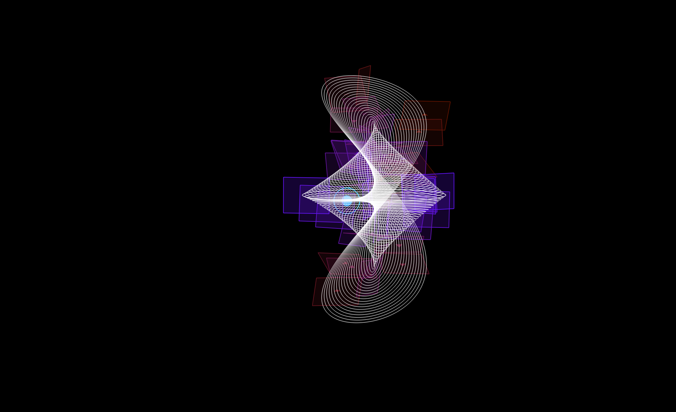
By running the script above, you should obtain a result similar to this.
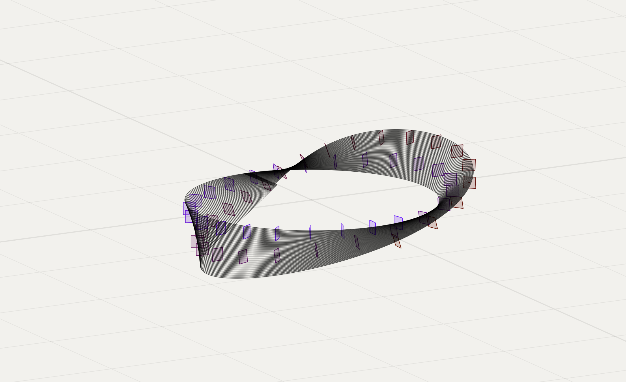
This render was done with Num_Curves = 50; each plane marker represents a cursor. From here, we can play the composition by using the playback transport on the bottom of the screen. Using this, we can speed up and slow down the performance playback, controlling the rate at which all cursors move through their parametric curves. With a working system for generating meaningful data, we can now export it to create interesting performances.
Communicating with an Outside Application
IanniX has a few available protocols for exporting data outside of the program including serial, MIDI, and UDP. This project uses OSC, as it is the most straightforward for communication between applications. To enable OSC communication in IanniX, go to the CONFIG tab in the inspector panel and select ENABLE OSC. Then specify the network ID and enter the receiving application’s OSC address. For this project, I used Csound as the audio engine, however this can be replaced with any audio generation program that can receive OSC messages.
Communicating with Csound
OSC communication in Csound is done by using the OSClisten opcode, in conjunction with the OSCinit opcode. The init function is called along with the OSC network ID to create a variable handle to the network, this handle is then passed to any OSClisten opcode (or other OSC protocol opcodes) to identify the OSC port.
mobius.csd
This section breaks down what’s happening in the .csd file without getting into too much Csound specifics. There are 3 instruments being used here: 2 of them are for retrieving data from the network (1 for the trigger data, 1 for the cursors), and the third one generates the actual audio.
Global Variables
At the top of the file, there is a range of global variables being initialized. Their descriptions describe their purpose, however the most important are the Cursor Values arrays. These arrays are initialized with space for each of the curves generated and will each hold a unique incoming data type (x-position, y-position, etc).
instr 1
instr 1 is responsible for retrieving the trigger data from the OSC network. Since the trigger data behaves much differently than the continuous cursor data, a separate instrument helps with clarity.
OSCListen
The trigger data is retrieved by using the opcode OSClisten. We pass both the global giPortHandle variable (initialized earlier) and the specific message address, along with the expected message format. IanniX automatically provides 4 message address types, and in this case we simply use the provided /trigger. We then provide the expected data format: in IanniX, trigger data can be configured to send lots of different data about the trigger, however in this case we are simply sending the trigger ID, along with the trigger value (127 when on, 0 when off), thus we provide the format ff. Finally, we provide the variables which the retrieved values will be stored in: ktid, and ktval.
The rest of instr 1 is dedicated to triggering a musical effect whenever the trigger fires. Although the OSClisten opcode returns a trigger value (here, kGotTrig), I found it more stable to use the changed opcode to trigger from the actual retrieved OSC value. When triggered, the variable ktval activates the conditional below, executing the musical logic. For the sake of brevity, I won’t get into the details of this logic, but the overall intended effect is to trigger a random transposition of each oscillator every 2.1 cycles around the Möbius strip.
instr 2
instr 2 serves a similar purpose to instr 1 in handling incoming data, however it requires a bit more precise programming to handle all of the incoming messages. Rather than collecting a single variable from one trigger, we now collect 5 data parameters from potentially 50+ continuous data curves. To solve this, we employ unique arrays for each variable, large enough to hold a parameter for each curve; we store data by cursor ID for easier data management; and we use a loop to retrieve messages and store them in their respective arrays.
The first loop uses Csound’s kgoto loop protocol. The OSClisten opcode is called once per k-rate cycle (default: every 48000/64 samples); each time this occurs, we loop through all cursors to ensure all data is updated properly. This loop does that by using the kGotIi variable to check for new messages (it will be 1 whenever there is a new message), and if so, takes the data collected in the variables provided to the OSClisten opcode, and stores them in their respective arrays. This repeats until there are no more new messages, in which case it exits.
Finally, the retrieved data is processed into a more meaningful format for use in instr 3.
instr 3
Finally, instr 3 takes the data collected from instr 1 and instr 2 and generates the audio. This instrument creates a simple sine wave oscillator for each curve, mapping cursor x, y, and z positions to frequency, amplitude, and filter parameters. The main audio generator is the oscili opcode, which receives the amplitude data, processed frequency data, and a custom waveshape to produce a tone.
Running an Instrument Loop
In order to create a unique oscillator for each curve, a loop was employed. However, creating a loop of unique audio-rate instruments proved tricky in Csound. The solution uses a recursive loop via the schedule opcode. We can find this loop at the very bottom of instr 3.
if(p4 + 1 < giNumBands) then
	schedule(3, 0, p3, p4+1)
endif
By calling itself, this opcode continuously instantiates new instances of instr 3. Using p-variables, we pass the ID value to each new instrument instance, closing the loop once sufficient instruments have spawned; this variable also indexes into the positional data arrays generated by IanniX.
Audio Process
The actual audio processing happing in instr 3 is relatively simple. First, the oscili opcode generates a sine wave using the processed amplitude and frequency data (The frequency data includes an extra processing step to detune certain frequencies based on the y-variable). The audo is then scaled down based on the number of total oscillators and a basic low-pass filter is applied, using more positional data to feed the frequency and resonance. Finally, the oscillators are panned across the stereo field evenly using the cursor ID. That is the entire audio generation process, however some more data processing was done to ensure oscillator frequencies were consonant. Mapping the cursor x-position to raw frequencies leads to a very dissonant jumble of noise; to make the piece more musical, position data intended for frequencies were first mapped onto a custom musical scale in the array: giNotes[], which outlines an extended chord structure with alternating major and minor thirds, with an extra major second on top.
giNotes[] fillarray -3, 0, 4, 7, 11, 14, 16
Transposing via Trigger
The trigger data collected in instr 1 is used to create a random transposition effect on the oscillators periodically throughout the performance. This is achieved by feeding the processed trigger signal from instr 1 into a random generator that produces integer values between -3 and 3. This value is stored in a global variable and retrieved within instr 3. Whenever the trigger signal is activated, it updates the transposition value in instr 3, and this value is sent to all the oscillators, transposing the entire musical effect at the same time. A portk opcode was also added to create a glide between the new notes when a new transposition occurs.
Score Editor
Lastly, we need to instruct our instruments to run when we press play. This is done by adding a score in the Score Editor. Note that instrument 3 requires an extra argument, p4, that represents our curve/instrument ID, which we pass a value of 0.
i1 0 1000
i2 0 1000
i3 0 1000 0
Running the System
Once both files are properly set up, to run the complete performance with both applications, we simply need to press play in both the IanniX transport system and Csound. If OSC communication is properly set up, then we should be able to hear our array of oscillators panned across the stereo field, shifting notes in seemingly random ways.
Debugging Communication Issues
If the Csound file plays but the tones are static, then this means it isn’t receiving the data from IanniX. If this happens, ensure both IanniX and the OSCinit opcode are using the same host/network; sometimes the OSC system in Csound can be a little buggy, so it can be useful to use an OSC monitoring application for debugging.
Interacting with the Performance
Now that the performance is running, we can use the param_ variables implemented in the Möbius strip equation to alter both the visual shape being displayed and the data sent to Csound, thereby changing the produced sound. In IanniX, under Inspector > Objects, select our group of cursors, then go to the info tab in the inspector to access the parameter sliders. By moving these sliders, we update the variables within the equation, and IanniX will in turn update the curves and cursors. By incorporating 5 different parameters, we can mangle the shape in many interesting ways, creating unique visual and audio effects.
Note: Changing parameters will cause the OSC data to update immediately, often resulting in harsh jumps in the audio output. The best way to address this is by using an opcode like portk in Csound to smooth out abrupt changes during audio processing, rather than trying to buffer or delay the OSC messages (unless you’re specifically aiming for lower-resolution OSC communication).
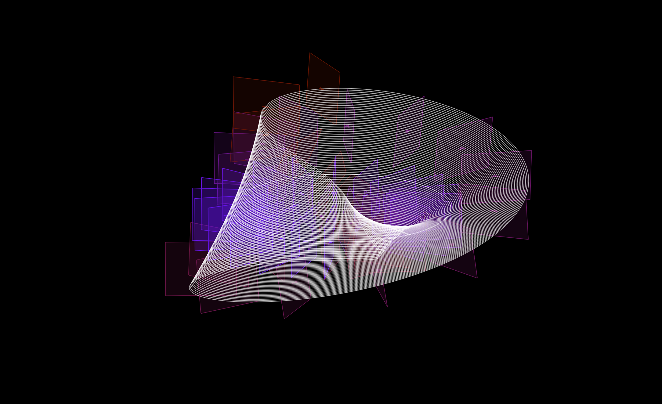
Below are some visual results from experiments with changing the parameters:
Moving Cursors
Another useful feature of IanniX, especially for this project, is the ability to set cursor start positions. Within a cursor’s settings in the inspector, we can adjust some of the time-based behavior of individual cursors. This is great for creating variance between cursors that follow similar paths.
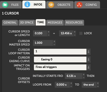
In addition to the inspector panel, these options can also be set via the script editor. For instance, in this project, when all cursors start at the same position, the generated audio is almost identical across oscillators. While it is interesting to hear the subtle detuning that occurs as the cursors gradually diverge, we might prefer a more chaotic result right from the start. We can use the script editor to offset the starting positions of the cursors at the beginning of the performance. In this example, a loop is employed and the following command is executed for each curve:
run("setoffset current " + offset + " 0 0");
This instructs the currently selected curve to start at an offset determined by the offset variable, which increments on every loop pass. The result is an even distribution of cursors spread further around the Möbius curve, ordered by their IDs. However, there are many other interesting ways to distribute the cursors—for example, by adjusting their speeds (an approach not explored in this project, but one that would likely yield interesting results).
Conclusion
The purpose of this project was to experiment with IanniX and explore the capabilities of using a graphical data system to control an audio engine, specifically Csound. I found the project very successful in producing an interesting visual and musical performance. Learning IanniX was straightforward, and I encountered no major issues with the script editor or overall workflow. The biggest challenge was configuring Csound to properly retrieve OSC data from IanniX. With continuous data streaming constantly, it required a loop and array storage to handle reliably; but now that a working example exists, it should help future enthusiasts get started more quickly.
Despite the initial hurdles, the project resulted in a truly interesting performance system. Using a loop to draw curves that outline a 3D shape proved fascinating, both as a visual effect and as a rich source of musical data. Incorporating programmable param_ variables into the parametric equations also led to unexpected and exciting consequences: real-time alteration of the curves transforms IanniX from a static composition tool into a dynamic live performance instrument. I’m very interested in extending this project toward more interactive, live-based applications.
Csound proved to be an effective and powerful audio engine for this setup. Retrieving the OSC data was tricky at first, but with a working example in place, it becomes straightforward to connect any Csound synthesis technique to data transmitted from IanniX. This project relies on basic opcodes, focusing on layering many simple tones to create its overall effect. However, Csound offers opcodes for virtually any synthesis process, so there are countless ways the audio could be extended and enriched.
The combination of IanniX and Csound creates a unique and engaging system for both performer and audience. If you have any interest in digital audio, data sonification, and/or 3D visuals, I highly recommend trying these tools out for yourself.